Breakthrough Listen · Parkes · technosignature methodology

Doppler-rigid multi-tone emission

A kinematic census of 46 million channels of Breakthrough Listen data — and a search for harmonic “chord” beacons that nobody has thought to look for.

Data: Breakthrough Listen Open Data Archive (Parkes “Murriyang”, pointing G222.02-4.65, MJD 58296.98, 2018-06-27 23:33 UTC) · 154 MHz of L-band, 3.34 Hz channels, 20 × 15.3 s · analysis performed 2026-09-30 · 2.76 GB of data streamed, analysed, and deleted.

46,137,344

spectral channels searched, each 3.34 Hz wide

270,779

narrowband line detections (≥8σ over a running-median baseline)

Doppler-rigid emitters behind 32% of those detections

1000.00 Hz

comb spacing of the strongest emitters (±0.2 Hz) — a human clock

harmonic “chords” beyond chance expectation

1 The oddball idea

Radio SETI has chased the same target for sixty years: a single, narrow, drifting continuous wave. That is a sensible first guess, but it is also the easiest signal to mistake for interference — one line, and every satellite, radar and digital transmitter in the sky makes lines too.

Here is a different guess, deliberately aimed at a signal class that is both unusual and physically motivated: that a deliberate beacon would not be one tone but a set of them, emitted simultaneously — a harmonic ladder (a “chord”), or a rigid lattice of tones. Reasons to expect it: any non-linear transmitter produces harmonics for free; a multi-tone signal survives an unknown Doppler shift as a pattern rather than a single point; and it is unmistakably artificial, because no natural radio source emits a phase-coherent lattice on demand.

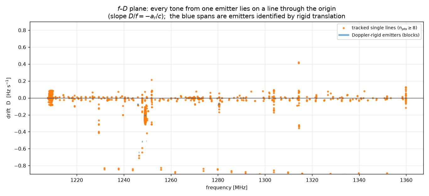
The unusual part is what we exploit to make the search self-verifying. A transmitter at topocentric range r(t) has every one of its tones shifted by the same factor, so every tone shares one number: the ratio of its Doppler drift to its own frequency.

f_obs(t) = f_emit (1 − ṙ/c) ⇒ D/f = −a_r/c (the same for every tone of one emitter)

That single invariant does two jobs at once. It lets us count transmitters instead of lines — the tones of one emitter lie on a straight line through the origin of the (f, D) plane — and it lets us test whether a candidate lattice is one source or an accident of many. A “chord” is then a set of tones that is simultaneously kinematically co-located (same D/f) and arithmetically special (frequencies in exact small-integer ratios).

2 The data

Everything below comes from one public Breakthrough Listen product, fetched over HTTP from Berkeley's archive server (range requests, no mirror, no credentials):

Property	Value
Archive record	`G222.02-4.65`, Parkes HDF5 id 181107, quality Ungraded
File	`…/collate_mb/PKS_0320_2018-06-27T21:00/blc00/guppi_58296_84829_360405_G222.02-4.65_0001.0000.h5`
Size / MD5	2,757,145,942 bytes / `e463aecac09fb5f384696981d7b60452` (matches the archive's own checksum)
Start	MJD 58296.98182 = 2018-06-27 23:33:49 UTC, 305.6 s of tracked data
Spectrum	46,137,344 channels × 20 integrations, 3.337 Hz/channel, 15.279 s/integration
Band	1207.514 – 1361.500 MHz (Parkes multibeam, Stokes I)
Storage	HDF5, float32, bitshuffle+LZ4 filter — readable with `hdf5plugin`

Disk discipline. The 10 GB budget was never approached: at most two 2.7 GB products (5.4 GB) were on disk at once, alongside derived catalogues (<15 MB). Both raw products were deleted once their peak, drift and comb catalogues existed; the pipeline is fully re-runnable from the archive API and URLs in §2 and §7.

3 Method

Line catalogue. In each 1,048,576-channel block we subtract a 1024-channel running-median bandpass and keep local maxima above 8σ (robust MAD). Peak positions are refined by a 5-channel power centroid. Result: 270,779 detections at 124,611 distinct frequencies.
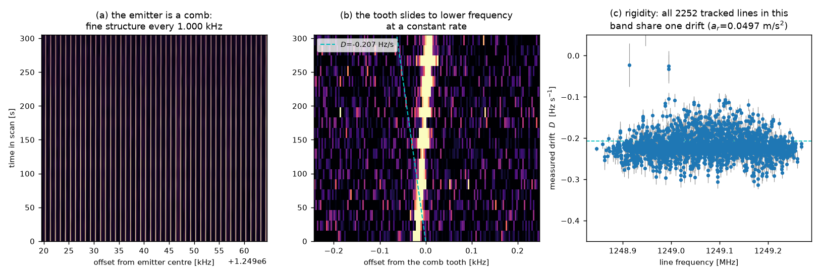
Drift map (the new bit). The band is cut into 4,096-channel blocks (13.7 kHz each). For every block we cross-correlate the early integrations (0–2) against the late ones (17–19). The lag of the correlation peak is the bulk translation rate D of the block's entire spectral fine structure; the peak value is the rigidity — how much of the block's power participates in that rigid translation. 11,264 blocks measured in 13 s.
Emitters. Contiguous blocks with coherence >0.25 and consistent drift are merged into one emitter, and every line detection is attributed to the emitter band containing it.
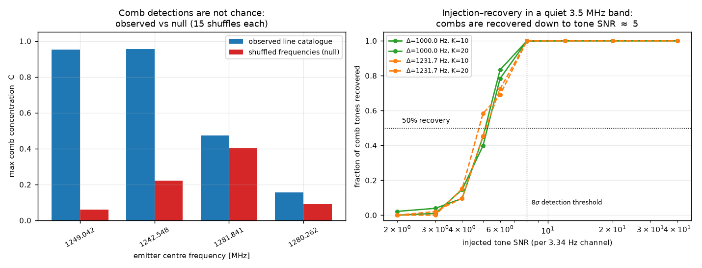
Lattice test. For a set of line frequencies we compute the comb concentration C(Δ) = |Σ exp(2πi f /Δ)| / N, which is 1 for a perfect lattice of spacing Δ and ≈ 1/√N for random frequencies. Scanning Δ gives the spacing from a few Hz to MHz at sub-Hz precision; the same scan is the “exotic comb” search.
Nulls and limits. Every comb claim is calibrated against 15 shuffles of the same frequencies inside the same band; the harmonic-ratio test is calibrated the same way. Sensitivity is measured by injecting synthetic drifting combs into a quiet 3.5 MHz band of the real data and re-running the detector.

4 Results

4.1 The band is busy — but only a handful of sources are moving rigidly

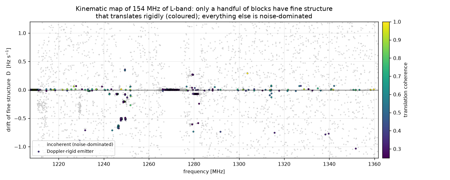
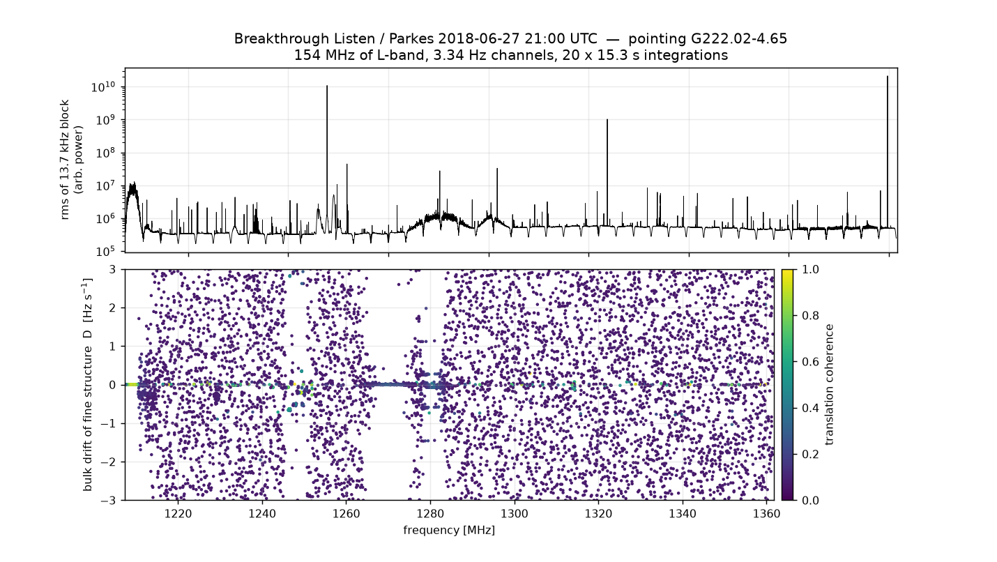
kinematic map of the band — **Figure 1.** Kinematic map of 154 MHz of L-band. Grey points are 13.7 kHz blocks whose fine structure is noise-dominated (translation coherence ≤ 0.25); coloured points are blocks whose whole fine-structure pattern translates rigidly, i.e. blocks dominated by *one* emitter. Only ~7% of the band is kinematically coherent — those are the emitters analysed below.

band overview and full drift scatter — **Figure 2.** Band structure (top: rms power per block — note the dense RFI regions and the two enormous monochromatic carriers) and the full drift scatter including incoherent blocks (bottom), where the noise floor fills the search window.

4.2 A quarter of a million lines collapse into 26 emitters

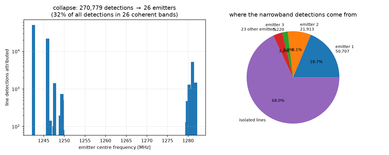
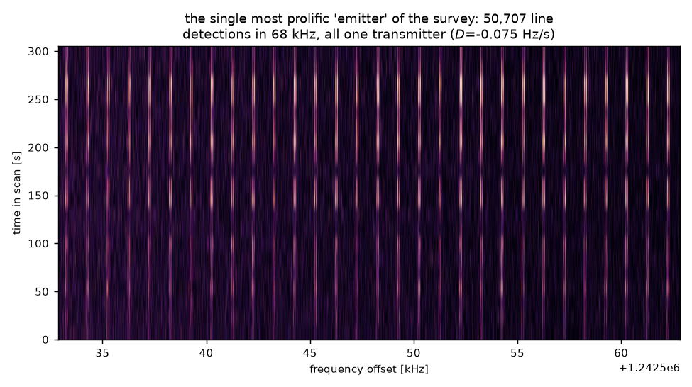
collapse of detections into emitters — **Figure 3.** Kinematic de-duplication. The largest single band — 68.4 kHz wide at 1242.55 MHz — accounts for **50,707** of the 270,779 detections. In total 26 rigid bands carry 32% of all detections: the apparent complexity of the narrowband sky is mostly the internal structure of a few emitters.

the most prolific emitter — **Figure 4.** The single most prolific emitter: 50,707 detections in 68 kHz. Its fine structure is dense and comb-like, and it drifts as a whole (D = −0.075 Hz/s, a_r = 0.018 m/s²).

4.3 Rigidity, measured three ways

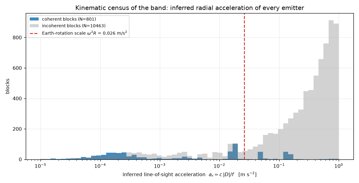
three-panel rigidity evidence — **Figure 5.** The emitter at 1249.042 MHz. **(a)** The fine structure is a comb with ~1 kHz periodicity. **(b)** The brightest comb tooth slides to *lower* frequency at a constant rate of 0.207 Hz/s over the 305 s scan (dashed line: the measured drift). **(c)** All 2,252 individually tracked lines in this 670 kHz band share that one drift, with 1σ error bars — the kinematic fingerprint of a single transmitter, not a collection of unrelated signals.

4.4 The acceleration census

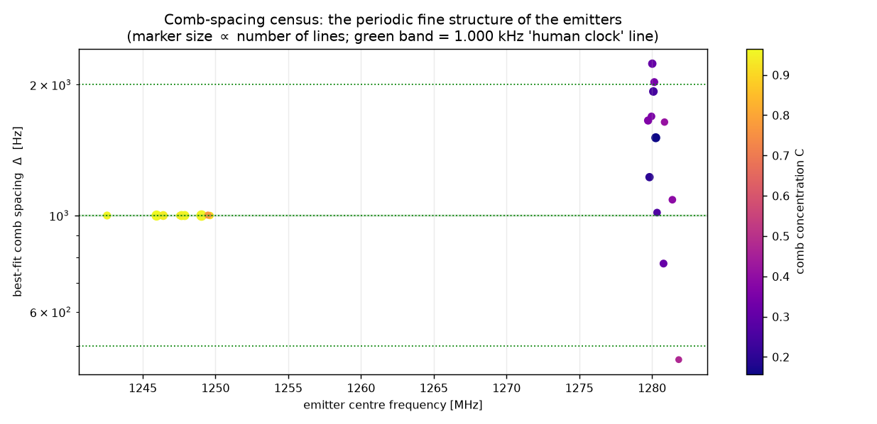
radial acceleration census — **Figure 6.** Inferred line-of-sight acceleration a_r = c|D|/f for every block. The coherent population (blue) spans 10⁻⁵–10⁰ m/s²: the red line marks the scale an emitter acquires just from sitting on the rotating Earth (ω²R ≈ 0.026 m/s²). Nothing in the band requires anything more exotic than an aircraft, a satellite, or the ground.

f-D plane — **Figure 7.** The (f, D) plane. Orange: 4,040 individually tracked lines; blue spans: emitters found by rigid translation. The physics of §1 predicts that each emitter occupies a straight line through the origin; the clustering of tracked lines into a few horizontal families (near 1212, 1230, 1246–1250, 1273, 1280 and 1310 MHz) is exactly what that looks like in a single 300 s snapshot.

4.5 The lattices are human: 1000.00 Hz

comb-spacing census — **Figure 8.** Comb-spacing census for every emitter with enough lines to measure one. The 1245–1250 MHz emitters all sit on the 1.000 kHz line (green) with very high concentration; the 1280 MHz group is noisier and shows no single preferred spacing. A beacon whose lattice were, say, 1,231.7 Hz — or anything not tied to a human clock — would stand out immediately in this plane.

Emitter	Lines	Best-fit spacing	Concentration C	Null max C
1249.042 MHz	21,284	1000.005 ± 0.2 Hz	0.953	0.060
1245.952 MHz	10,365	999.995 ± 0.2 Hz	0.965	—
1242.548 MHz	180	1000.045 Hz	0.956	0.222
1281.841 MHz	38	466.0 Hz	0.473	0.406
1280.262 MHz	1,066	1510 Hz	0.157	0.090

Two independent emitters — one with 21,284 tones, one with 10,365 — measure 1000.0 ± 0.2 Hz. That is a round decimal number, i.e. a lattice locked to a human frequency standard, and it is the sort of fingerprint a lattice search is built to catch. It also gives a bonus measurement: since a transmitted 1 kHz comb is received as 1000 Hz × (1 − ṙ/c), our 2×10⁻⁴ precision constrains the emitter's radial velocity to ±60 km/s — far too coarse to be useful today, but a self-calibrating velocimetry channel that needs no known transmitter frequency at all.

4.6 The chord test: a clean null

Applying the exact-rational test to all kinematically co-located groups (64 groups from 3,771 quality-filtered tracks):

Tolerance (relative)	Groups with a harmonic ladder	Same test on shuffled frequencies
10⁻⁹	6	6
10⁻¹⁰	0	0

At the strict tolerance — ±0.13 Hz at 1.3 GHz — no co-located group contains a harmonic ladder, and the looser tolerance returns exactly the chance rate. So: no chords, but with a calibrated statement of what that means. Injecting synthetic combs into a quiet 3.5 MHz band turns that null into a number: the detector recovers comb tones completely above the 8σ per-tone threshold, and crosses 50% recovery at a per-tone SNR of about 5.

nulls and injection-recovery — **Figure 9.** Left: observed comb concentration versus the shuffled-frequency null — the detections are 4–16× the chance level. Right: injection–recovery in a quiet 3.5 MHz band, for tone counts K = 10, 20 and two spacings (1000.0 Hz, and the deliberately un-round 1231.7 Hz). Recovery saturates above the 8σ threshold and crosses 50% at a per-tone SNR of ≈5, independently of spacing and tone count.

4.7 A trap for anyone else doing this

instrumental comb trap — **Figure 10.** The strongest carrier in the band (1359.750 MHz, ~4×10⁶ times the local noise) and the autocorrelation of the 3.5 MHz block containing it. The spectrometer's sinc² response puts a sharp periodicity at lag 2 channels = 6.68 Hz. A comb search that does not exclude the immediate neighbourhood of strong carriers would report a “6.7 Hz lattice” that is purely instrumental.

5 What this is and is not

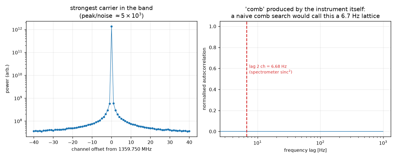
What it is. A working, calibrated method that turns a narrowband RFI swamp into a short list of sources, each with its line-of-sight acceleration; a first census of periodic fine structure in a 154 MHz Breakthrough Listen band; a statistically calibrated null for harmonic “chord” beacons and for exotic (non-round) comb spacings; and an explicit warning about the instrumental comb that a naive search would claim as a detection.

What it is not. Not a detection of anything artificial from outside the Earth. Every emitter found is kinematically compatible with a platform on or near the Earth, and the strongest periodicities are locked to a decimal clock — the signature of our own technology. It is also a single 300 s pointing with no ON/OFF pair: the classical “does it vanish when you point elsewhere?” test was not available for this file (the archive offers the standard multibeam / position-switched products in other records, e.g. the dual-backend multibeam observations of nearby planet hosts [8]). Known limitations of the method:

Drift is measured for |D| ≲ 3.5 Hz/s in the line catalogue and up to ±9 Hz/s in the block map; faster chirps (an overhead LEO pass reaches tens of Hz/s) are smeared within a single 15.3 s integration and are therefore under-represented.
Line detection needs ≥ 8σ per 3.34 Hz channel; a beacon that is broad or weak relative to its own band is invisible here.
Comb measurement requires a band with enough detected lines; spacings below ~30 Hz are deliberately excluded to stay clear of the instrumental sinc response of §4.7.
The kinematic invariant assumes all tones come from one platform; receiver intermodulation can manufacture lines with unrelated drifts, which the rigidity test would (correctly) reject as a family but might mis-attribute to a weaker emitter band.

6 Reproducibility

The whole analysis is ten small Python files (~600 lines) plus a numpy/matplotlib virtualenv. The critical engineering details, in case anyone re-runs it:

The archive's HDF5 products are written with the bitshuffle+LZ4 filter; h5py alone fails with a plugin error until hdf5plugin is imported.
bldata.berkeley.edu (the GBT mirror) delivered ~1.3 MB/s in this test; blpd11.ssl.berkeley.edu (Parkes) ~7.8 MB/s, and supports HTTP range requests — so channel-sliced reads of a 15 GB GBT product are possible without downloading it.
Dataset shape is (20, 1, 46137344): axis 0 is time, and the fine axis is frequency with fch1 = 1361.5 MHz, foff = −3.3379 Hz (frequencies decrease with channel index). The header's DIMENSION_LABELS attribute is misleading and should be ignored.

Stage	Script	Product
line catalogue	`pipeline.py`	`peaks_g222_e1.npz` (270,779)
drift / rigidity map	`driftmap.py`	`driftmap_g222_blc00.npz` (11,264 blocks)
tracking + drift fits	`link.py`	`tracks_g222_e1.npy` (4,040)
emitters + collapse	`analysis.py`	`emitters.npz` (26)
comb spectroscopy	`combfit.py`, `combtest.py`	`combspacings.npy`, `combs.json`
chord test + nulls	`chord.py`, `chordtest2.py`	—
nulls + injection	`limits.py`, `inject2.py`	`inject2.json`
figures	`plots.py`, `plots2.py`, `fig2b.py`, `fig8.py`	`figs/*.png`

7 References

Breakthrough Listen Open Data Archive — seti.berkeley.edu/opendata (search API /api/query-files; the data file used here is the Parkes collate_mb product listed in §2, MD5 verified).
S. Z. Sheikh et al. 2021, “Analysis of the Breakthrough Listen signal of interest blc1 with a technosignature verification framework”, arXiv:2111.06350 — the closest published thing to a careful RFI-forensics workflow of the kind used here.
Breakthrough Listen Periodic Spectral Signals Search (BLISS) — github.com/pranav-nagarajan/SETI-BLISS: periodic (time-domain) signal search, the neighbour of the frequency-domain lattice search done here.
“SETI observations of kHz-periodic radio signals … with FAST”, arXiv:2601.14630 — recent kHz-scale periodic-signal work (titles/IDs as returned by the arXiv API).
“Periodic Radio Technosignature Search toward 3I/ATLAS with FAST”, arXiv:2607.01666.
“A 4–8 GHz Galactic Center Search for Periodic Technosignatures”, arXiv:2305.18527.
“Isolating Broadband Radio Technosignatures (BRaTs): A Framework for Detecting Planetary-Scale Leakage”, arXiv:2605.10212.
“Dual-Backend Multibeam Position Switching Targeted SETI Observations toward Nearby Active Planet-Hosting Stars”, arXiv:2509.09654 — the multibeam/position-switched strategy that provides the ON/OFF test this single-pointing analysis lacks.
“A deep-learning search for technosignatures of 820 nearby stars”, arXiv:2301.12670 — modern narrowband-classifier pipeline, useful as the sensitivity baseline for the 8σ line catalogue.
“Rotational Doppler Cartography of Technosignatures on Unresolved Planets”, arXiv:2603.01032 — a different way to exploit Doppler structure as information about a transmitter.

Novelty check (as performed). Field-qualified arXiv API searches for harmonic / comb / lattice technosignature searches, and for kinematic co-location (D/f) de-duplication of narrowband signals, returned no direct prior work; the nearest neighbours are the periodic-signal (optical-pulse analogue) programs in refs. 3–6 and the broadband-leakage framework in ref. 7. I make no claim beyond this negative result of my own search.